Domo arigato, Mr. Roboto, Mata ah-oo hima de Domo arigato, Mr. Roboto, Himitsu wo shiri tai
Every once in a while an analyst is called upon to look at things that are unique, that pique the interest and make the day go by faster. (For other days, there is coffee.) As the web server admin approached my desk, I was just about to put on another pot of coffee. I decided to hold off.
Our admin came to me with a bit of a puzzle. Although there are a myriad of well-known robots spidering our website daily, there was one that he was not happy with. It was called Yandex, a Russian search engine. Given the amount of malware and other less-than-wanted things coming out of Russian networks, the admin was concerned about this indexer accessing our website. With a grin a mile wide, I set aside the coffee and reached for my green tea with honey, and responded with a heartfelt, “I’m on it.”
FIRST STEPS
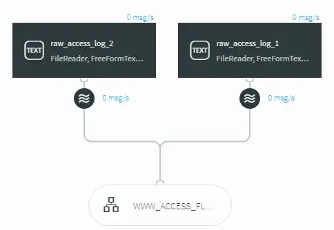
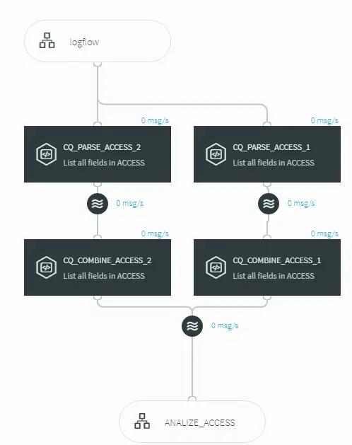
The first thing I needed to do was to get our web logs into a place where I could use Striim to analyze them. At my request, the admins had implemented SYSLOG-NG and were using a central repository for all of our logs which made it far easier to access them using Striim. Our primary and backup web servers in production resided in /var/log/www-prod-1 and /var/log/www-prod-2 on the central logging system. From there all I had to do was get them into Striim and we could start having fun. From the UI I whipped up a pair of text readers and configured them to take data from the access logs from both production servers.
The next step was to parse the log files so that the information from the log files was organized into fields that could be processed. A little wave of the REGEX wand and we had both logs parsed, and combined into a single flow for Striim to analyze.
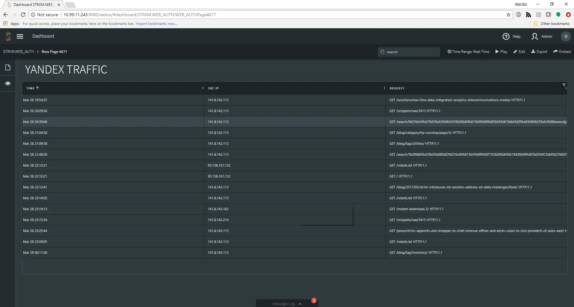
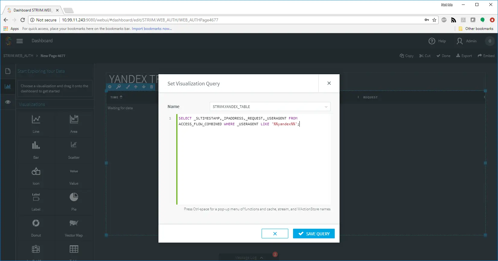
From there, I next created a dashboard to show me just the information related to the web requests from Yandex. This would give me a clean and up-to-date view of the data I needed in real time. A quick TQL query combined with a table and I was on my way!
Immediately the information started flowing in. At first, it looked like just normal traffic one would expect from a indexing spider bot. Sure enough, however, my keen eyes spotted something that was not quite right.
As Dorothy Parker would say, “What fresh hell is this?” The spider was making a GET request of the search function of our website! This is not normal behavior for a spider if all it was doing was indexing our site. A little analyst magic performed on that request revealed it was using our own site search feature to look for “Fun HB Slot Machine” and the domain qpyl18.com. A quick check of this domain showed that it was [protected by Cloufflare ( Hi Otto! )], but that the origin server was having issues. A quick check of the IP addresses involved and my spidey-analyst senses were tingling.
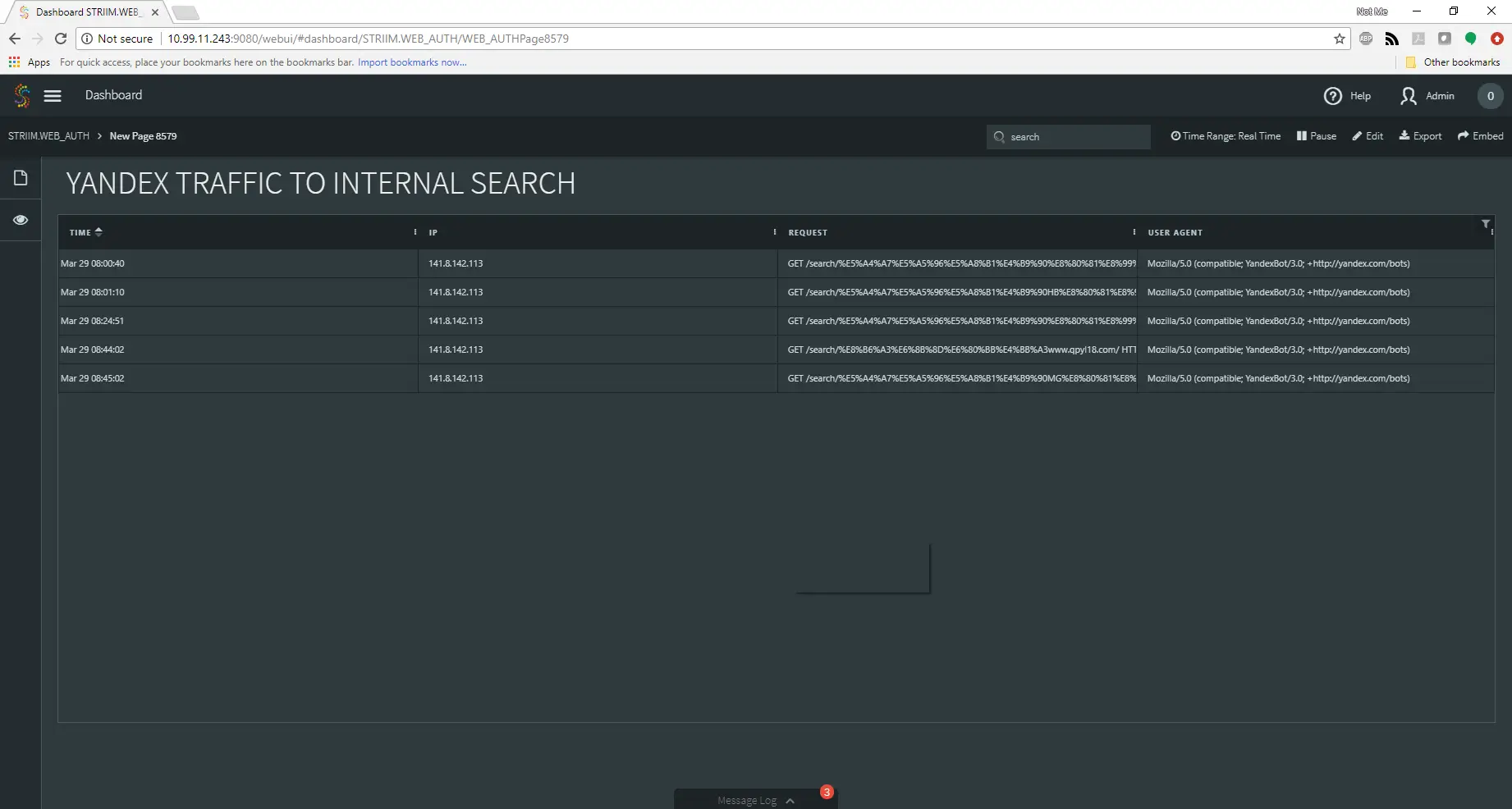
The next burning question was how often was this happening, and at what volume? Back to the dashboard I went! I altered my query to show me the requests that were performing the internal searches, and was quickly rewarded with the information I was looking for:
Not only was this happening, but it was happening frequently.
I configured Striim to keep a watch on this, making it part of my overall security application, and using customized queries to create indicators of how many instances in a day, average number of instances over a week, and a special dashboard page with alerts to let me know if it got out-of-hand.
Like any good analyst, I gathered data for 60 days and then presented it to the web admin, and we both decided this was not something we wanted on our network. A few adjustments to the web server, firewall, and IDS, and we were off for a celebratory lunch.
The ease of use, speed, and myriad of tools along with the flexibility of Striim allowed me and the web admin to quickly and efficiently acquire, process, enrich and report the data on the unusual traffic, and create an environment where any of the shift analysts could keep an eye on the activity, both streaming in real time and stored for historical purposes.
So you want to empower your analysts with tools like this? Request a demo today. We will be happy to guide you through all of the features of Striim and help you improve your security footprint.
In this series of blog-based tutorials, we are guiding you through the process of building data flows for streaming integration and analytics applications using the Striim platform. This tutorial focuses on SQL-based stream processing for Apache Kafka with in-memory enrichment of streaming data. For context, please check out Part One of the series where we created a data flow to continuously collect change data from MySQL and deliver as JSON to Apache Kafka.
In this tutorial, we are going to process and enrich data-in-motion using continuous queries written in Striim’s SQL-based stream processing language. Using a SQL-based language is intuitive for data processing tasks, and most common SQL constructs can be utilized in a streaming environment. The main differences between using SQL for stream processing, and its more traditional use as a database query language, are that all processing is in-memory, and data is processed continuously, such that every event on an input data stream to a query can result in an output.
The first thing we are going to do with the data is extract fields we are interested in, and turn the hierarchical input data into something we can work with more easily.
Transforming Streaming Data With SQL
You may recall the data we saw in part one looked like this:
This is the structure of our generic CDC streams. Since a single stream can contain data from multiple tables, the column values are presented as arrays which can vary in size. Information regarding the data is contained in the metadata, including the table name and operation type.
The PRODUCT_INV table in MySQL has the following structure:
LOCATION_IDint(11) PK
PRODUCT_IDint(11) PK
STOCKint(11)
LAST_UPDATEDtimestamp
The first step in our processing is to extract the data we want. In this case, we only want updates, and we’re going to include both the before and after images of the update for stock values.
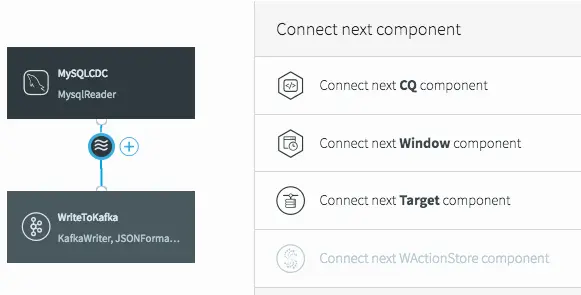
To do the processing, we need to add a continuous query (CQ) into our dataflow. This can be achieved in a number of ways in the UI, but we will click on the datastream, then on the plus (+) button, and select “Connect next CQ component” from the menu.
Connect Next CQ Component to Add to Our First Continuous Query
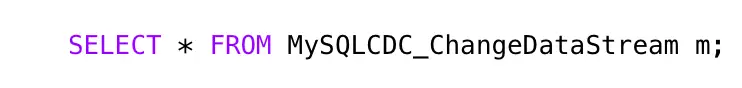
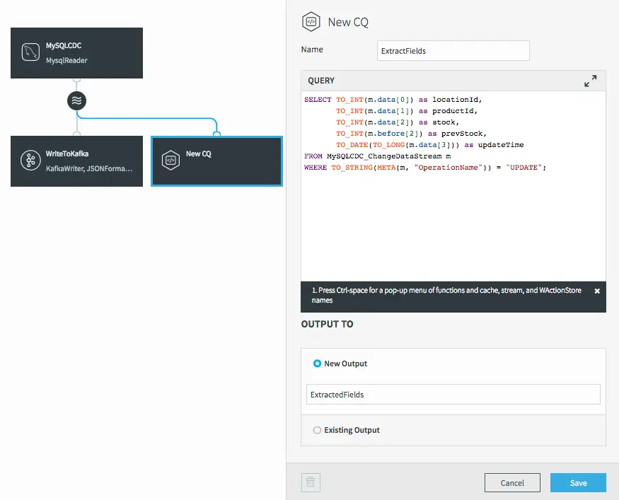
As with all components in Striim, we need to give the CQ a name, so let’s call it “ExtractFields”. The processing query defaults to selecting everything from the stream we were working with.
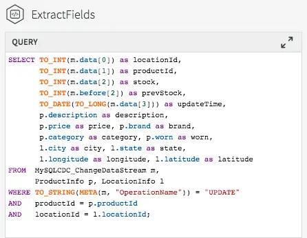
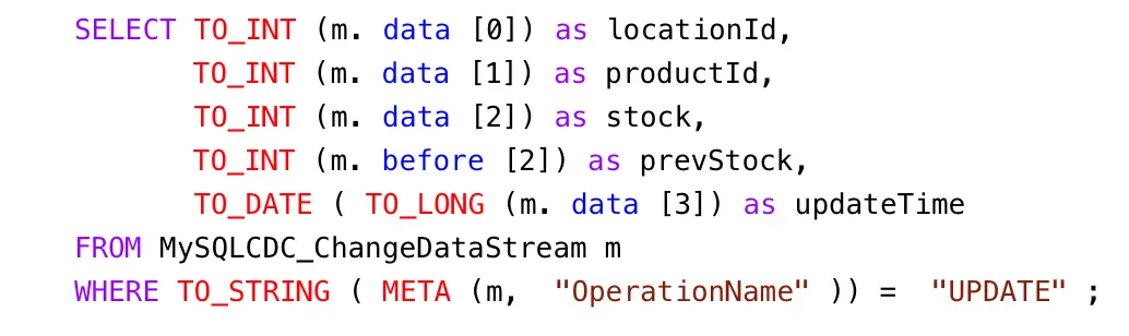
But we want only certain data, and to restrict things to updates. When selecting the data we want, we can apply transformations to convert data types, access metadata, and many other data manipulation functions. This is the query we will use to process the incoming data stream:
Notice the use of the data array (what the data looks like after the update) in most of the selected values, but the use of the before array to obtain the prevStock.
We are also using the metadata extraction function (META) to obtain the operation name from the metadata section of the stream, and a number of type conversion functions (TO_INT for example) to force data to be of the correct data types. The date is actually being converted from a LONG timestamp representing milliseconds since the EPOCH.
</code>
The final step before we can save this CQ is to choose an output stream. In this case we want a new stream, so we’ll call it “ExtractedFields”.
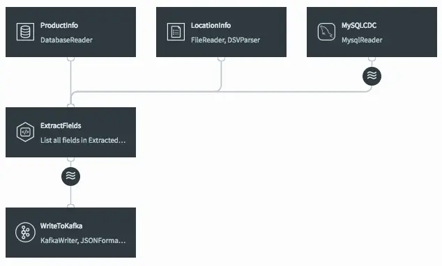
Data-flow with Newly Added CQ
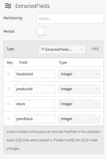
When we click on Save, the query is created alongside the new output stream, which has a data type to match the projections (the transformed data we selected in the query).
After Clicking Save, the New CQ and Stream Are Added
The data type of the stream can be viewed by clicking on the stream icon.
Stream Properties Showing Generated Type Division
There are many different things you can do with streams themselves, such as partition them over a cluster, or switch them to being persistent (which utilizes our built-in Apache Kafka), but that is a subject for a later blog.
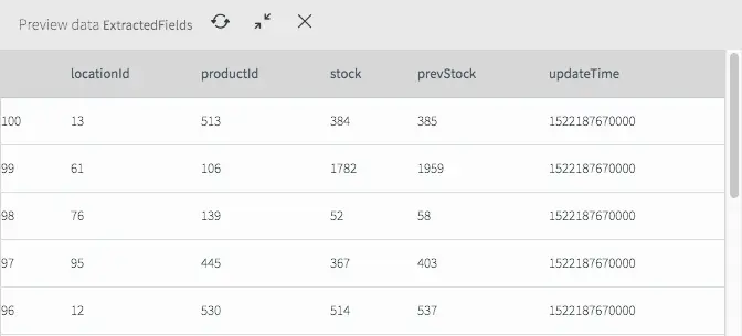
If we deploy and start the application (see the previous blog for a refresher) then we can see what the data now looks like in the stream.
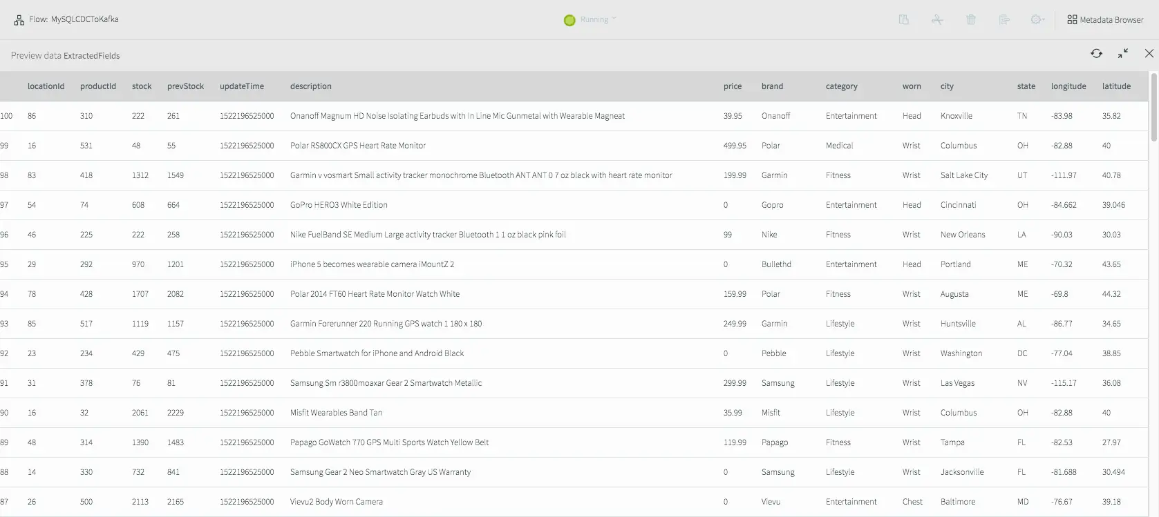
Extracted Fields Viewed by Previewing Data Streams
As you can see it looks very different from the previous view and now only contains the fields we are interested in for the remainder of the application.
But at the moment, this new stream currently goes nowhere, while the original data is still being written to Kafka.
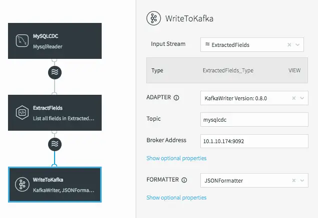
Writing Transformed Data to Kafka
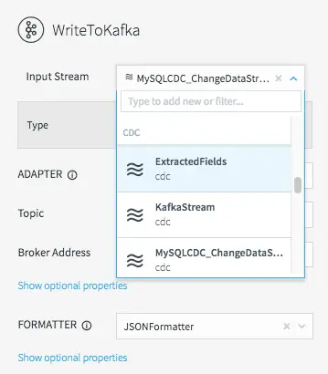
To fix this, all we need to do is change the input stream for the WriteToKafka component.
Changing the Kafka Writer Input Stream
This changes the data flow, making it a continuous linear pipeline, and ensures our new simpler data structure is what is written to Kafka.
Linear Data Flow Including Our Process CQ Before Writing to Kafka
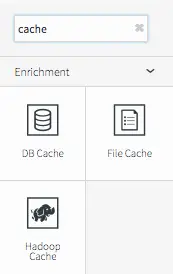
Utilizing Caches For Enrichment
Now that we have the data in a format we want, we can start to enrich it. Since the Striim platform is a high-speed, low latency, SQL-based stream processing platform, reference data also needs to be loaded into memory so that it can be joined with the streaming data without slowing things down. This is achieved through the use of the Cache component. Within the Striim platform, caches are backed by a distributed in-memory data grid that can contain millions of reference items distributed around a Striim cluster. Caches can be loaded from database queries, Hadoop, or files, and maintain data in-memory so that joining with them can be very fast.
A Variety of In-Memory Caches Are Available for Enrichment
In this example we are going to use two caches – one for product information loaded from a database, and another for location information loaded from a file.
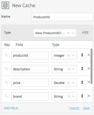
Setting the Name and Datatype for the ProductInfo Cache
All caches need a name, data type, lookup key, and can optionally be refreshed periodically. We’ll call the product information cache “ProductInfo,” and create a data type to match the MySQL PRODUCT table, which contains details of each product in our CDC stream. This is define in MySQL as:
PRODUCT_IDint(11) PK
DESCRIPTIONvarchar(255)
PRICEdecimal(8,2)
BRANDvarchar(45)
CATEGORYvarchar(45)
WORNvarchar(45)
The lookup key for this cache is the primary key of the database table, or productId in this case.
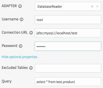
All we need to do now is define how the cache obtains the data. This is done by setting the username, password, and connection URL information for the MySQL database, then selecting a table, or a query to run to access the data.
Configuring Database Properties for the ProductInfo Cache
When the application is deployed, the cache will execute the query and load all the data returned by the query into the in-memory data grid; ready to be joined with our stream.
Loading the location information from a file requires similar steps. The file in question is a comma-delimited list of locations in the following form:
Location ID, City, State, Latitude, Longitude, Population
We will create a File Cache called “LocationInfo” to read and parse this file, and load it into memory assigning correct data types to each column.
Setting the Name and Datatype for the LocationInfo Cache
The lookup key is the location id.
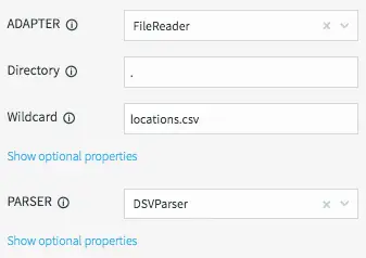
We will be reading data from the “locations.csv” file present in the product install directory “.” using the DSVParser. This parser handles all kinds of delimited files. The default is to read comma-delimited files (with optional header and quoted values), so we can keep the default properties.
Configuring FileReader Properties for the LocationInfo Cache
As with the database cache, when the application is deployed, the cache will read the file and load all the data into the in-memory data grid ready to be joined with our stream.
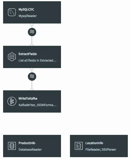
Dataflow Showing Both Caches Currently Ready to be Joined
Joining Streaming and Cache Data For Enrichment With SQL
The final step is to join the data in the caches with the real-time data coming from the MySQL CDC stream. This can be achieved by modifying the ExtractFields query we wrote earlier.
Full Transformation and Enrichment Query Joining the CDC Stream with Cache Data
All we are doing here is adding the ProductInfo and LocationInfo caches into the FROM clause, using fields from the caches as part of the projection, and including joins on productId and locationId as part of the WHERE clause.
The result of this query is to continuously output enriched (denormalized) events for every CDC event that occurs for the PRODUCT_INV table. If the join was more complex – such that the ids could be null, or not match the cache entries – we could change to use a variety of join syntaxes, such as OUTER joins, on the data. We will cover this topic in a subsequent blog.
When the query is saved, the dataflow changes in the UI to show that the caches are now being used by the continuous query.
Dataflow After Joining Streaming Data with Caches in the CQ
If we deploy and start the application, then preview the data on the stream prior to writing to Kafka we will see the fully-enriched records.
Results of Previewing Data After Transformation and Enrichment
The data delivered to Kafka as JSON looks like this.
{
“locationId“:9,
“productId“:152,
“stock“:1277,
“prevStock“:1383,
“updateTime“:”2018-03-27T17:28:45.000-07:00”,
“description“:”Dorcy 230L ZX Series Flashlight”,
“price“:33.74,
“brand“:”Dorcy”,
“category“:”Industrial”,
“worn“:”Hands”,
“city“:”Dallas”,
“state“:”TX”,
“longitude“:-97.03,
“latitude“:32.9
}
As you can see, it is very straightforward to use the Striim platform to not only integrate streaming data sources using CDC with Apache Kafka, but also to leverage SQL-based stream processing and enrich the data-in-motion without slowing the data flow.
In the next tutorial, I will delve into delivering data in different formats to multiple targets, including cloud blob storage and Hadoop.


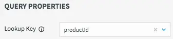 The lookup key for this cache is the primary key of the database table, or productId in this case.