In this demo, you’re going to see how you can utilize Striim to do real-time collection of change data capture from Oracle Database and deliver that, in real-time, into Microsoft Azure SQL Server. I’m also going to build a custom monitoring solution of the whole end-to-end data flow. (The demo starts at the 1:43 mark.)
Unedited Transcript:
Today, see how you can move data from Oracle to Azure SQL Server running in the cloud in real time using Striim and change data capture. So you have data in lots of article tables on premise and you want to move this into Microsoft Azure SQL Server in real time. How do you go about doing this without affecting your production databases? You can’t use SQL queries because typically these would be queries against a timestamp like table scans that you do over and over again and that puts a load on the Oracle database and you can also skip important transactions. You need change data capture, and CDC enables non-intrusive collection of streaming database change stream provides change data capture as a collector out of the box. This enables real time collection of change data from Oracle SQL server and my sequel. The CDC works because databases write all the operations that occur into transaction logs, change data capture listens to those transaction logs and instead of using triggers or timestamps, it directly reads these logs to collect operations.
This means that every DML operation, every insert update and delete is written to the logs captured by change data capture and turned into events by our platform. So in this demo you’re going to see how you can utilize Striim to do real time collection of change data capture from your Oracle database and deliver that in real time into Microsoft Azure SQL server. Also going to build the custom monitoring solution, the whole end to end data flow. First of all, connect to Microsoft Azure SQL server. In this instance we have two tables, t customer and t cost odd that we can show here are currently completely empty.
We’re going to use a data flow that we’ve built in Striim to capture data from a on premise Oracle database using change data capture. You can see some of the configuration properties here and deliver that. After doing some processing into Microsoft Azure SQL Server and you can see the properties for configuring that here. To show this, we’re going to run some SQL against Oracle and the SQL does a combination of inserts, updates and deletes against our two Oracle tables. When we run this, you can see the data immediately in the initial stream. That data stream is then split into multiple processing steps and then delivered into Azure SQL server. If we redo the query against Azure tables here, you can see that the previously empty tables now have data in them and that data was delivered and will continue to be delivered live as long as changes are happening in the Oracle database. In addition to the data movement, we’ve also built a monitoring application complete with dashboard that shows you the data floating through the various tables, the types of operations are occurring and the entire end to end transaction leg. This is the difference between when a transaction was committed on the source system and when it was captured and applied to the target and also some of the most recent transactions. This was built again using a data flow within the Striim platform.
This data flow uses the original streaming change data from the Oracle database and then the place of processing in the form of SQL queries to generate statistics. In addition to generating data for the dashboard, you can also use this as rules to generate alerts for thresholds, etc. And the dashboard itself is not hard coded. It’s generated using our dashboard builder, which utilizes queries to connect to the backend. Each visualization you’re seeing here is powered by a query. It’s the back end data, and there are lots of visualizations to choose from. So you’ve hoped you’d have enjoyed seeing how to move Oracle data on premise into the cloud using Striim.
In this blog post, we’re going to tackle the basics behind what streaming integration is, and why it’s critical for enterprises looking to adopt a modern data architecture. Let’s begin with a working definition of streaming integration.
What is Streaming Integration?
You’ve heard about streaming data and streaming data integration and you’re wondering, why is it an essential part of any enterprise infrastructure?
Well, streaming integration is all about continuously moving any enterprise data with real high throughput in a scalable fashion, while processing that data, correlating it, and analyzing it in-memory so that you can get real value out of that data, and visibility into it in a verifiable fashion.
And streaming data integration is the foundation for so many different use cases in this modern world, especially if you have legacy systems and you need to modernize, you need to use new technologies to get the right answers from your data, and you need to do that continuously, in real time.
Why Streaming Integration?
Now that we’ve outlined a high-level understanding of what streaming integration is, let’s discuss why it’s important. You now know streaming integration is an essential part of enterprise modernization. But why? Why streaming integration and why now?
Well, streaming data integration is all about treating your data the way it should be treated. Batch data is an artifact of technology and technology history – that storage was cheap, and memory and CPU were expensive. And so, people would store lots of data and then process it later.
But data is not created in batches. Data is created row-by-row, line-by-line, event-by-event as things in the real world happen. So, if you’re treating your data in batches, you’re not respecting it; you’re not treating it the way that it’s created. In order to do that, you need to collect that data and process it as it’s being produced, and do all of this in a streaming fashion. And that’s what streaming integration is all about.
If you’re interested in learning more about streaming data integration and why it’s needed, please visit our Real-Time Data Integration Solution page, or view the wide variety of sources and targets that Striim supports.
How to build change data capture into Kafka and do some processing on that, and then do some delivery into other things. So this is pure integration play. You start off by doing change data capture from MySQL. In this case, MySQL would build the initial application and then configure how you get data from the source so we can figure the information to connect into MySQL. When you do this, we’ll check and make sure everything is going to work right, that you already have change data capture configured properly. And if it wasn’t, how you have to fix it and how to do it. You don’t select the tables that you’re interested in. We’ve got to collect the change data, and this is going to create a data stream, but then go to two different to Kafka.
So we’re going to configure how we want to write into Kafka, and that’s basically setting up what the broker configuration is, what the topic is and how we want to format the data. In this case, we’ve got to write to add as JSON, when we save this, this is gonna create a data flow. And the data flow is very simple. In this case, it’s two components. We go in from MySQL CDC source into a Kafka writer. We can test this by deploying the application. And it’s a two stage process. You deploy it first, which will put all the components out over the cluster and then you run it. And now we can see the data that’s flowing in between. So if I click on this, I can actually see the real time data and you see there’s a data and there was it before.
That’s basically the before updates. You get the before image as well, so you can see what’s actually changed. So this is real time data flowing through the MySQL application, the raw data may not be that useful. And one of the pieces of data in here is a product ID. And that probably doesn’t contain enough information, so what we’re going to do first is we’re going to extract the various fields from this and those various fields include the location ID products, id, how much stock there is, et cetera. This is an inventory monitoring table and we just turned that from kind of a raw array format into a set of name fields. So it’ll make it easier to work with later on. And you can see the structure is very different. Now what we’re actually seeing in that data stream, if we then add additional context to this, what we’ll be able to do is join that data with something else. So first of all, we’ll just configure this so that instead of writing the raw data add to Kafka, we’ll write that process state ad. And you can see all we have to do is change the input stream. So that will change the data flow. Now are write process data into Kafka.
But now we go into add a cache and this is a distributed in memory data grid that’s going to contain additional information that we want to join with our raw data. And so this is product information. So every product ID is a description and price and some other stuff. So first of all, we just create a data type that corresponds to our database table. Configure what the keys and the key in this case is the product Id. Then we specify how are we going to get the data. And it could be from files, it could be from HDFS. We’re going to use a database reader to load it from MySQL table. So especially specify all the connections and the query we’re going to use. And we now have a cache of products information to use this, we modify as SQL to just join in the cache. So anyone that’s ever written any SQL before knows what a join looks like. We’re just joining on the product Id. So now instead of just the raw data, we now have these additional fields that we’re pulling in in real time from the product information. So if we start this and look at the data again, you will actually be able to see the additional fields like description and brand and category and price that came from that other type that’s all joined in memory. There’s no database lookups going on is actually really, really fast.
If you already have data on Kafka or another message bus or anywhere else for that matter is new files, you may want to kind of read it and push at some of the targets. So what we’re going to do now is going to take that data we just wrote to Kafka. We’re going to use Kafka reader in this case. So it will just search for that and track the source and then we can configure that with the properties connect to the broker that we just used. So because we noticed JSON data, we’re going to use a Jason parser. I was going to break it up into a adjacent object structure. And then create this data stream. Okay, when we deploy this and start this application, it’ll start reading from that Kafka a topic.
Well, we can look at that data and we can see this is the data that we were writing that previously with all the information in it and it’s adjacent full Max. You can see the adjacent structure though. So the other targets that we go into right to the JSON structure might not work. So what were you going to do now is build a query that’s going to pull the various fields, edit that JSON structure and creates a well-defined data stream that has various individual fields in it. So a variety crew to do that. It’s directly accessing the JSON data and saves that. And now instead of the original data stream that we had with the JSON in it, when we deploy this, start it up and looked at the data, and this is incidentally how you would build applications, looking at the data all the time, as you’re building on adding additional components into it. If we’re looking at the data stream now, then you’d be able to see that we have those individual fields, which is what we had before on the other side of Kafka, but don’t forget that it may not be stream to Kafka. It could be anything else. And if you were doing something like we just did with CDC into Kafka than Kafka into additional targets, you don’t have to have Kaftan in between. You can just like take the CDC and push it out to the targets directly.
So, uh, what are we going to do now is going to add a simple target, which is going to write to a file. And we do this by choosing the file adopt. So the fall reuter and especially finding the format we want. So we are gonna write this. I’ve seen the CSV format. We actually call it DSV because it’s delimiter separated. And the limits could be anything. It doesn’t have to be a coma and save that. And now we have something that’s going to right out to the file. So if we deploy this and start this up, then we’ll be creating a file with real-time data.
And after a while it’s got some data in it and then we can use something like a Microsoft Excel to actually view the data to check that it’s kind of what we wanted. So let’s take a look in Excel and we can see the data that we initially collected from MySQL be written to capita being slightly from Kafka and then being and back out into the CSV file. They just have one target and a single data flow, or you can, it’s multiple targets if you want. We’re going to add to, in rising into Hadoop and into Azure Blob Storage. So what we do is in the case of Hadoop, we don’t want all the data to go to a dud. So as a simple CQ to restrict the data and do this by location id. So when location 10 is going to be written to do, that’s so some filtering going on there.
And now we will add in the Hadoop target. So you’re gonna write to HDFS as a target, drag that into the data flow and see there’s many ways of working the platform. We also have a scripting language by the way, that enables you to do all of this from vi or emacs or whatever your favorite attack status or is. And we’re going to write to HDFS. I see an Avro format, so it will specify the scheme of file. And then when this is started up, we’ll be writing into HDFS as well as to this local file system. And similarly, if we want to write into Azure Blob Storage, we can take the adaptive for that and just search for that and drag that in from the targets. And we’ve got to do that on the original source data, not that query. So we’ll drag it into a, that original data stream.
Okay. And now we just configure this with information from Azure. So you need to find out what is the URL, and you should know what your key is and the username and password and things like that. You go into collect that information if you don’t have it already. And then add that into the target definition for your Azure Blog Storage. I’m gonna write that out in JSON format. So that’s kind of very quickly how you can do real time streaming data integration with our platform. And all of that data was streaming. It was being created by doing changes to MySQL.
I recently gave a presentation on operationalizing machine learning entitled, “Fast-Track Machine Learning Operationalization Through Streaming Integration,” at Intel AI Devcon 2018 in San Francisco. This event brought together leading data scientists, developers, and AI engineers to share the latest perspectives, research, and demonstrations on breaking barriers between AI theory and real-world functionality. This post provides an overview of my presentation.
Background
The ultimate goal of many machine learning (ML) projects is to continuously serve a proper model in operational systems to make real-time predictions. There are several technical challenges practicing such kind of Machine Learning operationalization. First, efficient model serving relies on real-time handling of high data volume, high data velocity, and high data variety. Second, intensive real-time data pre-processing is required before feeding raw data into models. Third, static models cannot achieve high performance on dynamic data in operational systems even though they are fine-tuned offline. Last but not the least, operational systems demand continuous insights from model serving and minimal human intervention. To tackle these challenges, we need a streaming integration solution, which:
Filters, enriches and otherwise prepares streaming data
Lands data continuously, in an appropriate format for training a machine learning model
Integrates a trained model into the real-time data stream to make continuous predictions
Monitors data evolution and model performance, and triggers retraining if the model no longer fits the data
Visualizes the real-time data and associated predictions, and alerts on issues or changes
Striim: Streaming Integration with Intelligence
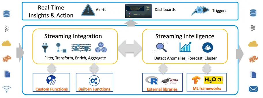
Figure 1. Overview of Striim
Striim offers a distributed, in-memory processing platform for streaming integration with intelligence. The value proposition of the Striim platform includes the following aspects:
It provides enterprise-grade streaming data integration with high availability, scalability, recovery, validation, failover, security, and exactly-once processing guarantees
It is designed for easy extensibility with a broad range of sources and targets
It contains rich and sophisticated built-in stream processors and also supports customization
Striim platform includes capabilities for multi-source correlation, advanced pattern matching, predictive analytics, statistical analysis, and time-window-based outlier detection via continuous queries on the streaming data
It enables flexible integration with incumbent solutions to mine value from streaming data
In addition, it is an end-to-end, easy-to-use, SQL-based platform with wizards-driven UI. Figure 1 describes the overall Striim architecture of streaming integration with intelligence. The architecture enables Striim users to flexibly investigate and analyze their data and efficiently take actions, while the data is moving.
Striim’s Solution of Fast-Track ML Operationalization
The advanced architecture of Striim enables us to leverage it to build a fast-track solution for operationalizing machine learning. Let me walk you through the solution in this blog post using a case of network traffic anomaly detection. In this use case, we deal with three practical tasks. First, we detect abnormal network flows using an offline-trained ML model. Second, we automatically adapt model serving to data evolution to keep a low false positive rate. Third, we continuously monitor the network system and alert on issues in real time. Each of these tasks correspond with a Striim application. For a better understanding with a hands-on experience, I recommend you download the sandbox where Striim is installed and these three applications are added. You can also download full instructions to install and work with the sandbox.
Abnormal network flow detection
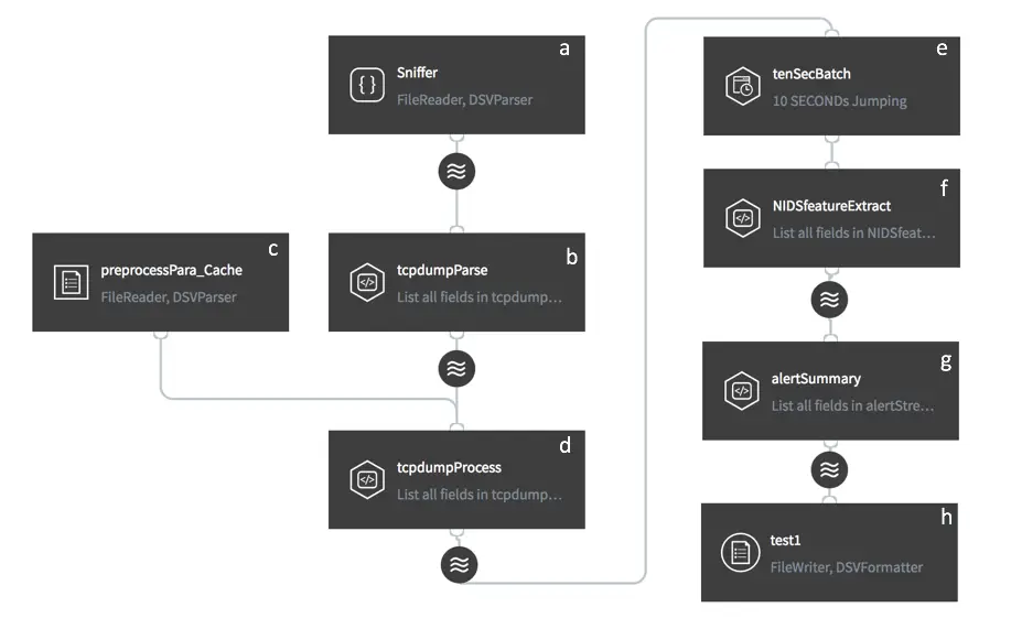
Figure 2. Striim Flow of Network Anomaly Detection
We utilize one-class Support Vector Machine (SVM) to detect abnormal network flows. One-class SVM is a widely used anomaly detection algorithm. It is trained on data that has only one class, which is the normal class. It learns the properties of normal cases and accordingly predict which instances are unlike the normal instances. It is appropriate for anomaly detection because typically there are very few examples of the anomalous behavior in the training data set. We assume that there is an initial one-class SVM model offline trained on historical network flows with specific features. This model is then served online to identify abnormal flows in real time. This task requires us to perform the following steps.
Ingest raw data from the source (Fig. 2 a);
For ease of demonstration, we use a csv file as the source. Each row of the csv file indicates a network flow with some robust features generated from a tcpdump analyzer. Striim users simply need to designate the file name, and the directory where the file locates, and then select DSVParser to parse the csv file. These configurations can be written in a SQL-based language TQL. Alternatively, Striim web UI can navigate users to make the configurations easily. Note that you can work with virtually any other source in practice, such as NetFlow, database, Kafka, security logs, etc. The configuration is also very straightforward.
Filter the valuable data fields from data streams (Fig. 2 b);
Data may contain multiple fields, and while not all of them are useful for the specific task, Striim enables users to filter the valuable data fields for their tasks using standard SQL within continuous query (CQ). The SQL code of this CQ is as below, where 44 features plus a timestamp field are selected and converted to the specific types, and an additional field “NIDS” is added to identify the purpose of data usage. Besides, we pause for 15 milliseconds at each row to simulate continuous data streams.
SELECT “NIDS”,TO_DATE(TO_LONG(data[0])*1000), TO_STRING(data[1]), TO_STRING(data[2]), TO_Double(data[3]),TO_STRING(data[4]),TO_STRING(data[5]),TO_STRING(data[6]),TO_Double(data[7]),TO_Double(data[8]), TO_Double(data[9]),TO_Double(data[10]),TO_Double(data[11]),TO_Double(data[12]),TO_Double(data[13]),TO_Double(data[14]),TO_Double(data[15]),TO_Double(data[16]),TO_Double(data[17]),TO_Double(data[18]),TO_Double(data[19]),TO_Double(data[20]),TO_Double(data[21]),TO_Double(data[22]),TO_Double(data[23]),TO_Double(data[24]),TO_Double(data[25]),TO_Double(data[26]),TO_Double(data[27]),TO_Double(data[28]),TO_Double(data[29]),TO_Double(data[30]),TO_Double(data[31]),TO_Double(data[32]),TO_Double(data[33]),TO_Double(data[34]),TO_Double(data[35]),TO_Double(data[36]),TO_Double(data[37]),TO_Double(data[38]),TO_Double(data[39]),TO_Double(data[40]),TO_Double(data[41]),TO_Double(data[42]),TO_Double(data[43]),TO_Double(data[44]) FROM dataStream c WHERE PAUSE(15000L, c)
Preprocess data streams (Fig. 2 c, d);
To guarantee SVM to perform efficiently, the numerical features need to be standardized. The mean and standard deviation values of these features are stored in cache (c) and used to enrich the data streams output from b. Standardization is then performed in d.
Aggregate events within a given time interval (Fig. 2 e);
Suppose that the network administration does not want to be overwhelmed with alerts. Instead, he or she cares about a summary for a given time interval, e.g., every 10 seconds. We can use a time bounded (10-second) jumping window to aggregate the pre-processed events. The window size can be flexibly adjusted according to the specific system requirements.
Extract features and prepare for model input (Fig. 2 f);
Event aggregation not only prevents information overwhelming but also facilitates efficient in-memory computing. Such an operation enables us to extract a list of inputs, where each input contains a specific number of features, and to feed all inputs into the analytics model to get all of the results once. If analytics is done by calling remote APIs (e.g., cloud ML API) instead of in-memory computing, aggregation can additionally decrease the communication cost.
Detect anomalies using an offline-trained model (Fig. 2 g);
We utilize one-class SVM algorithm from Weka library to perform anomaly detection. A SVM model is first trained and fine-tuned offline using historical network flow data. Then the model is stored as a local file. Striim allows users to call the model in the platform by writing a java function specifying model usage and then wrapping it into a jar file. When there are new network flows streaming into the platform, the model can be applied on the data streams to detect anomalies in real time.
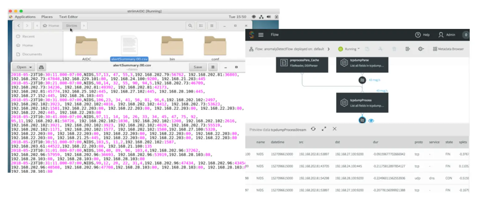
Persist anomaly detection results into the target (Fig. 2 h).
The anomaly detection results can be persisted into a wide range of targets, such as database, files, Kafka, Hadoop, cloud environments etc. Here we choose to persist the results in local files. By deploying and running this first application, you will see the intermediary results by clicking each stream in the flow and see the final results continuously being added in the target files, as shown in Fig. 3.
In part 2 of this two-part post, I’ll discuss how you can use the Striim platform to update your ML models. In the meantime, please feel free to visit our product page to learn more about the features of streaming integration that can support operationalizing machine learning.